
Dr. Robert Gebotys 2006
1
Chapter 10: Regression Analysis
Read
: Chapter 10 then read the notes and try
the WEBCT assignment questions. If you need
more practice, try the practice questions with
answers available on the web.
Exercises:
Introduction
In Chapter 2 you were introduced to the method
of least squares regression. This was a
technique of fitting a line model to data. In the
next several chapters the common techniques of
inference were introduced and developed. Two
of the most common inference methods were
the test of hypothesis and confidence intervals.
In this chapter the techniques of inference are
applied to the line so that inferences can be
made about the unknown parameters, the slope
and intercept.
View the Video - Inference for Relationships

Dr. Robert Gebotys 2006
2
Review Chapter 2 Material
In this chapter we add tests of significance and
confidence intervals to our line model
introduced in Chapter 2. Thus, we begin with a
brief review of that material. We now write the
line as: y = B
o
+ B
1
x
This is the equation of a straight line. It is in
contrast to y=a+bx, the notation in Chapter 2.
B
1
and B
o
are the parameters or unknowns in
the line.
B
o
is the y-intercept, the value of y when x=0.
B
1
is the slope or how y changes per unit
increase in x.
Example: Consider the following line
y = 2 + 6x
When x = 0, y = 2; therefore the y-intercept = 2.
When x increases 1 unit, y increases by 6. In
other words, the slope = 6.
Dr. Robert Gebotys 2006
3
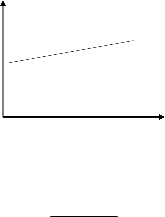
In order to plot the line, pick 2 points that are on
the line, say (0,2) the y-intercept and (3,20).
!
!!
!
(3,20)
!
!!
!
y (0,2)
0 x
Suppose a researcher has a graph of x vs y for a
number of points.
In chapter 2 we saw that the best fitting line was
calculated using least squares. In other words,
deviations in the vertical direction are used to
select the line.
Dr. Robert Gebotys 2006
4
In other words the line that minimizes
deviations in the vertical direction is the best
line:
ŷ
i
= b
0
+ b
1
x
i
(read ŷ
i
as the predicted value of y by the line)
e
i
2
= (observed y - predicted y)
2
residual squared
The line that minimizes e
i
2
is the best line.
!
!!
!
!
!!
!
y
e
y
!
! !
! ŷ
!
!!
!
0
x

Dr. Robert Gebotys 2006
5
We use the following formulas to find the best
fitting line that minimizes the residuals about
the line. Note that a computer is used to find the
least squares regression
line in practice.
b
1
=
b
0
=
The researcher assumes that a line is an
appropriate model for the data collected on the
system under study.
The model is a line: y = B
o
+ B
1
x where
B
o
and B
1
are unknown population parameters.
The sample data are used to make inferences
about the population parameters.
∑ (x
i
– x ) (y
i
– y )
∑ (x
i
– x )
2
y –
b
1
x
Dr. Robert Gebotys 2006
6
In this problem, the data are viewed as
composed of 2 parts:
Data = Model (fit) + Error (residual)
y = (b
o
+b
1
x) + e
From the data we make inferences about the
population. The data give the researcher sample
estimates of the population parameters. Using
the information in the sample, inferences are
made concerning the population.
Data (y)
Model Error
sample b
o
+b
1
x e
Inference
population B
o
+B
1
x E
NOTE: We have only one response variable
(y) and one predictor variable (x) defined on a
population π. Our response variable y is
quantitative.

Dr. Robert Gebotys 2006
7
Based on the observed values of the predictor
variable (x) we want to construct a line which
we will use to predict values of y.
Example: Gebotys & Roberts (1987), CJBS,
examined two variables, age of a person in years, and
how that person views the seriousness of a crime as
recorded on a scale where a higher number indicates
more seriousness. The sample data for 10 randomly
sampled people are given below. The population of
interest is all people in Ontario over the age of 18.
age (x) serious (y)
20 21
25 28
26 27
25 26
30 33
34 36
40 31
40 35
40 41
80 95
A line is assumed an appropriate model for this problem.
Dr. Robert Gebotys 2006
8
The means are: x = 36 y = 37.3
The least squares estimates for the slope and
intercept are:
b
1
= 1.197
b
0
= y - b
1
x = –5.792
Our equation is then y = 5.792 + 1.197x. A plot
of the data confirms the researcher’s assumption
that a line is a reasonable model to consider for
this data.
!
!!
!
!!!
!!!!!!
!!!
y
!!!!!
!!!!!!!!!!
!!!!!
0 x
Use table 9.1 below to verify the slope and
intercept. In practice, these calculations are
done using a computer. The hand calculations
are given here for your information and better
understanding of the method.

Dr. Robert Gebotys 2006
9
Table 9.1
x
i
y
i
(x- x) (y- y) (x-x)
2
(y-y)
2
(x - x)
(y- y)
1 20 21 -16 -16.3 256 265.69 260.8
2 25 28 -11 -9.3 121 86.49 102.3
3 26 27 -10 -10.3 100 106.09 103.0
4 25 26 -11 -11.3 121 172-69 124.3
5 30 33 -6 -4.3 36 18.49 25.8
6 34 36 -2 -1.3 4 1.69 2.6
7 40 31 4 -6.3 16 39.69 .25.2
8 40 35 4 -2.3 16 5.29 -9.2
9 40 41 4 3.7 16 13.69 14.8
10 80. 95 44 57.7 1936 3329.29 2538.8
Totals 360 373 0 0 2622 3994.1 3138.0
x = 36 y = 37.3
The least squares estimate of B
1
the slope of the
line is:
b
1
= = = 1.197
∑ (x – x ) (y – y)
∑ (x – x )
2
3138
2622

Dr. Robert Gebotys 2006
10
A one unit increase in age (x) gives a 1.197
increase in the rating of crime seriousness (y).
The least squares estimate of B
0
, the y-intercept
of the line, is:
b
0
= y - b
1
x
= 37.3 – 1.197(36)
= -5.792
This completes a brief review of Chapter 2. We
now introduce inference for the line.
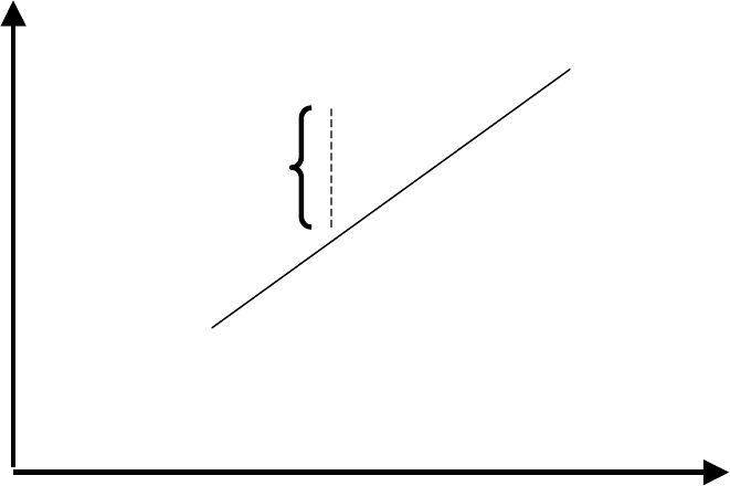
Inference for the Line
For the model y=B
o
+ B
1
x the population of y
values is assumed normally distributed about a
mean that depends on x.
We write E(y x) to read average value of y
given x to represent these means. We assume
the means lie on a line given by the equation of
a line. See the plots below.
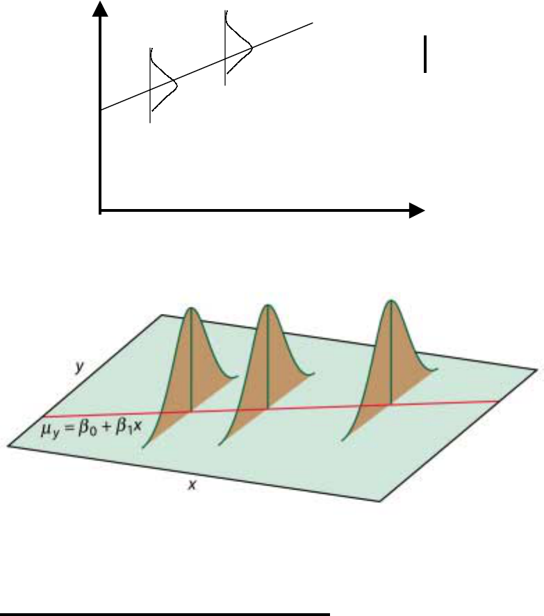
Dr. Robert Gebotys 2006
11
!
!!
!
E(y x) = B
o
+ B
l
x
y
!
!!
!
0 x
Figure 10.2
Properties of Residuals
The residuals (e
i
) are assumed to:
1) Be independent
2) Follow a normal distribution with
mean = 0
3) Have unknown variance equal to σ
2

Dr. Robert Gebotys 2006
12
We check 2) with a probability plot and
simulation.We estimate σ
2
the variance in the
population using s
2
our sample estimate.
The calculation of s depends on the residuals. If
residuals are large (poor fit of the data by a line)
then s will be large. Conversely, if they are
small (line a good model for the data), “s” will
be small. Table 9.2 is used to calculate s below:
Table 9.2
x
i
y
i
ŷ=b
0
+b
1
e
i
=y
i
- ŷ
i
e
i
2
1 20 21 18.15 2.85 8.12
2 25 28 24.13 3.87 14.98
3 26 27 25.33 1.67 2.79
4 25 26 24.13 1.87 3.50
5 30 33 30.12 2.88 8.29
6 34 36 34.91 1.09 1.19
7 40 31 42.09 -11.09 122.99
8 40 35 42.09 -7.09 50.27
9 40 41 42.09 -1.09 1.19
10 80 95 89.97 5.03 25.30
Dr. Robert Gebotys 2006
13
Totals 360 373 373.01 -0.01 238.62
s
2
= = = = 29.83
In other words, the spread, or variance, of the
residuals about the line is 29.83.
Researchers often report the square root of s
2
,s
the standard deviation since given the
assumption of normality some quick
calculations can be made about the residuals and
their distribution.
We know that ± 1 standard deviation for the
normal gives approximately 68% of the data. In
our example:
s = 5.46
so, plus or minus 5.46 will give approximately
68% of the data. Sometimes the residuals are
standardized, Z scores are created so that the
∑e
i
2
n - 2
238.62
10 - 2
Dr. Robert Gebotys 2006
14
rules learned in Chapter 1 concerning the
normal can easily be applied.
Standardized residuals greater than 3 or less
than -3 are called outliers
.
Let us examine our sample variance formula
which we use to estimate our population
variance given below:
S
2
= =
n-2 is called the degrees of freedom
We subtract 2 from our sample size since we
want to estimate 2 parameters (B
o
,B
1
) or
unknowns.
σ
2
is the spread of the observations about the
line in the population.
∑e
i
2
n - 2
∑ (y-ŷ)
2
n - 2

Dr. Robert Gebotys 2006
15
Tests of Significance & Confidence Intervals:
We previously spoke of significance tests and
confidence intervals for the t distribution in
Chapter 7.
In general we saw that the test of hypothesis that
a parameter equals zero has the following form:
estimate
T = standard error of the estimate
If the sample size is large or the variance known
we could use a z test to perform our test of
significance. Usually, however, the variance is
unknown and the sample size small (n<50).
For the slope of our line we have the following
test of hypothesis:
H
o
: B
1
= 0 (x is not related to y)
H
a
: B
1
=/ 0 (x is related to y)
Dr. Robert Gebotys 2006
16
The test statistic is T, the sample slope over the
corresponding standard error, is given below:
T = b
1
s(b
1
)
The statistic is compared to the t-distribution
with n–2 degrees of freedom. If T is an
unreasonable value from the t distribution (i.e.,
p< .05) we have evidence against the null.
A 1 - α confidence interval for the slope is given
by:
b
1
± t
α/2
s(b
1
)
With the standard error is given by:
s(b
1
) = s/ √∑(x – x)
2

Dr. Robert Gebotys 2006
17
For example (continued)
We want to see if age and crime seriousness are
related, so a line model was fit to the data. To
confirm a relationship we want to test if the
slope of the line for the crime seriousness data is
zero. Our test of hypothesis is written as:
H
o
: B
1
= 0
(age & crime seriousness are NOT related)
H
a
: B
1
=/ 0
(age and crime seriousness ARE related)
We saw s = 5.46 from our previous calculation.
The standard error is:
s(b
1
) = 5.46/51.21 = .11
The t statistic is:
T = b
1
/s(b
1
) = 1.197/.11 = 10.88
with degrees of freedom n-2 = 10-2 = 8 df

Dr. Robert Gebotys 2006
18
The p-value is less than .0001 indicating we
have very strong evidence against the null
hypothesis. Therefore, we reject H
o
: B
1
= 0, and
conclude that age is useful in predicting a
judgement of crime seriousness.
A 95% CI for the slope is given by b
1
± t s(b
1
)
which is:
1.197 ± 2.306 (.11)
(.943, 1.451)
The slope of line in the population is between
.943 and 1.451 with 95% confidence.
Analysis of Variance for the Line
The total variation in “y” is divided into two
components (as before):
Data = Model + Error

Dr. Robert Gebotys 2006
19
= 1 + 2
1) amount of variance in the data
accounted for by the model (line)
2) amount of variance in the data NOT
accounted for by the model (line) or
error
If the model is good (i.e., there are small
residuals) then the model component should be
large and the error small.
We can write this data partitioning as a sums of
squares (SS):
SS Total = SS Model + SS Error
SST = SSM + SSE
∑ (y – y)
2
= ∑ (ŷ – y)
2
+ ∑ (y – ŷ)
2
The degrees of freedom associated with each
SS is:
1 for SSM since we are testing H
o
: B
1
=0

Dr. Robert Gebotys 2006
20
(1 parameter)
n-2 for SSE since there are 2 parameters
in model (B
o
, B
1
)
n-1 for SST since we do not test the y intercept
(i.e., H
o
: B
o
= 0 (one parameter))
Each component of 1) and 2) has a mean square:
MS = sum of squares (SS)
degrees of freedom (df)
For example:
MSE = SSE/ DFE
= ∑ (y – ŷ)
2
/ (n – 2)
= s
2
(an estimate of σ
2
)
To test:
H
0
: B
1
= 0

Dr. Robert Gebotys 2006
21
H
a
: B
1
≠ 0
Use an F-statistic:
F = MSM/MSE
Which will have an F (1, n-2) distribution under
the null hypothesis. If the model is not a good
one, our estimate of error is about the same size
as the effect of the model and we would expect
an F ratio equal to 1.0. On the other hand, if the
effect of the model is much larger than error, we
would expect the F-ratio to be > 1.0.
We report our results in an ANOVA table since
our estimates of model and error are based on
the amount of variance accounted for by each of
the two components:
Source Sums of
Squares
Degrees
of
Freedom
Mean
Square
F
Model ∑ (ŷ – y)
2
1
SSM/DFM MSM/MSE
Error ∑ (y – ŷ)
2
n – 2
SSE/DFE
Total ∑ (y – y)
2
n – 1

Dr. Robert Gebotys 2006
22
In the case of the line, the square of the
correlation coefficient (r) is:
R
2
= SSM/SST
This gives the proportion of variation in y
accounted for by x assuming a line model. What
is 1- R
2
? (hint write 1 as SST/SST.) R
2
was
first introduced in Chapter 2.
Example (cont’d)
For the Gebotys and Roberts (1987) data
construct an ANOVA table. Indicate how well
the model accounts for the data.
Refer to table 9.1 for SST:
SST = ∑ (y – y)
2
= 3994.1
See table 9.2 for SSE and SSM:
SSE = ∑ e
i
2
= 238.62
SSM = SST – SSE
Dr. Robert Gebotys 2006
23
= 3994.1 – 238.62
= 3755.48
since n = 10
DFM = 1
DFE = n-2 = 8
DFT = n-1 = 9
MSM = SSM = 3755.48 = 3755.48
DFM 1
MSE = SSE = 238.62 = 29.83
DFE 8
F = MSM = 3755.48 = 125.90
MSE 29.83

Dr. Robert Gebotys 2006
24
The results are summarized in an ANOVA table
below:
Source SS DF MS F
Model 3755.48 1 3755.48 125.90
Error 238.62 8 29.83
Total 3994.1 9
Note that the F statistic is equal to 125.90.
Since the OLS or p-value is <.0001 with 1, 8
degrees of freedom we have very strong
evidence against:
H
0
= B
1
= 0
and conclude there is a significant linear
relationship between age and seriousness.
An estimate of σ
2
, the spread about the line, can
also be easily calculated from the table since
s
2
=MSE = 29.83.
R
2
= SSM = 3755.48 = .94
SST 3994.1
Dr. Robert Gebotys 2006
25
In other words 94% of the variance in crime
seriousness (y) is accounted for by the model
(i.e., age). The model is adequate from an
ANOVA as well as percent variance accounted
for (R
2
) point of view. An examination of the
residuals is next.
In terms of proportion of variance in y
accounted for by x we have:
• R
2
= 0 if the model accounts for 0 variance.
• R
2
= 1 if the model accounts for all the
variance or perfect fit.
Researchers want models that account for a high
and significant amount of variance. Click SPSS
Example one to see the computer calculation of
the above statistics.
SPSS EXAMPLE ONE
The process of fitting a line is usually
accomplished with the help of a computer. In
Dr. Robert Gebotys 2006
26
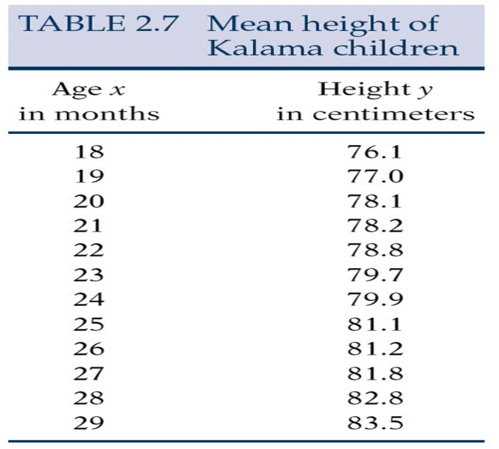
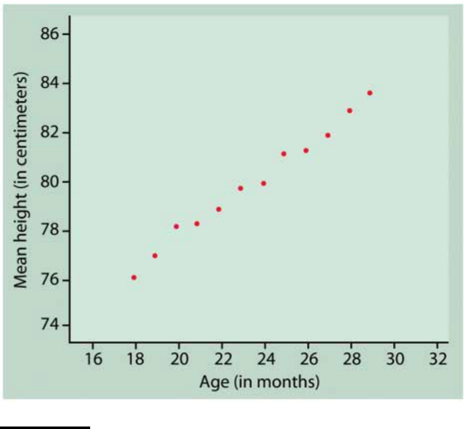
SPSS Example One, the data is analyzed using
SPSS. See the introduction to SPSS manual for
another example using the data below that
describes the relationship between children’s
age and height.
A graph of the data follows on the next page.
Dr. Robert Gebotys 2006
27
Example
A researcher is interested in seeing how oxygen
uptake and heart rate are related.
She suspects there is a linear relationship
between the two variables. The SPSS
commands in Chapter 2 show how to read and
Dr. Robert Gebotys 2006
28
plot the data. The plot below shows a clear
linear relationship.
.
.
. .
.
V02 .
.
HR
The following SPSS example shows how to
answer questions 1, 2, 3 below:
1) Fit a line to the data
2) Find 95% prediction intervals for heart rates
95 and 110
3) Construct residual plots to check
assumptions.

Dr. Robert Gebotys 2006
29
SPSS EXAMPLE TWO
Click SPSS example two above to view a
program that will answer the questions in the
example.
Summary
The model for simple linear regression has been
introduced. There are two unknowns in the
model or population parameters, the slope and
the intercept. From the data we calculate least
squares regression estimates of the parameters.
We use the sample estimates to make inferences
about the population parameters. Tests of
hypothesis and confidence intervals are
introduced using the t distribution.
The Analysis of Variance (ANOVA) table is
introduced to show how the data is split into two
pieces, model and error. If the model is not a

Dr. Robert Gebotys 2006
30
reasonable one then the F ratio
of model over
error components will equal 1.0.
Remember: Tips for Success
1) Read the text
2) Read the notes.
3) Try the assignment.
4) If needed, try the exercise questions.
5) Try the simulations and view the videos
if you need more help with a concept.
6) Try the self tests for practice on each
chapter of the text at:
www.whfreeman.com/ips
7) Steady Work = SUCCESS
